Photonics and Numerical Modeling: A look at Maxwell's Equations
Arti Agrawal
Thinking of photonics often conjures up pretty pictures of experiments with laser light and lab-coat clad scientists working with protective goggles on. The mental images usually in some way involve multi-million dollar equipment being used to produce exciting, cutting-edge results.
Many of these images are accurate and the array of experimental work in all the sub-disciplines that make up photonics are a testament to it.
I'd like to submit humbly that underlying all this fantastic and beautiful work is the theory of Classical Optics, encapsulated by 4 simple equations: the Maxwell's equations (see, open university, wiki ) presented by James Clerk Maxwell (and you can hear this programme on the BBC on Maxwell) in the 1860s.
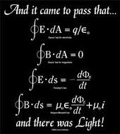
Einstein said of these equations, that: "The formulation of [Maxwell's] equations is the most important event in physics since Newton's time..."
The behaviour of all electromagnetic fields is governed by Maxwell's equations (in the classical limit). Therefore, all light and optical phenomena are a solution of these equations.
Whether we study how light travels in an optical fiber, reflection and absorption of sunlight at a solar cell surface, modes of optical resonators and cavities, Bragg gratings, band gaps in photonic crystals and many more: all of these devices/phenomena are described by solving Maxwell's equations. So they are fundamentally relevant to all of us with an interest in photonics.
This is where modeling and simulation become important too.
Fabricating a device is time consuming and very expensive. Plus, it’s almost impossible to get it right in the first attempt. This means several cycles of fabrication, testing, characterization, re-design, and finally, fabrication again.
Through numerical simulation, however, we can predict the optical properties of the proposed structure by simply solving Maxwell's equations (with appropriate boundary conditions) on a computer. This is obviously faster and cheaper than fabrication, and gives every optical designer and scientist a powerful tool: they can simulate the structure first and redesign numerically till they get the ideal, optimized structure before doing any fabrication.
This numerical solution approach also allows us to simulate optical behaviour in devices or situations that we cannot experimentally create with current technology. As the equations are scale invariant and work at all frequency ranges (that we know of), we can explore many different electromagnetic regimes with simulation tools. Thus solution of the Maxwell's can literally act as a telescope into the future with regards to future photonics developments.
Almost every research lab uses some sort of simulation or modeling software that does this work. Most of these software implement numerical techniques such as the FEM, FDTD, BPM (not an exhaustive list by any means) to solve the Maxwell's equations and obtain either the optical mode or evolution of the optical field/mode in the structure. From this, quantities such as power, loss, propagation constants, field overlap, Poynting vector, resonant frequency, bandwidth, transmission, reflection etc., can be calculated.
Here, I'd like to introduce a small caveat: numerical solutions to the Maxwell's equations are required where solutions through semi/analytical approaches are not possible. In fact in such situations, the only way to solve the equations is numerically.
So when you next think of an optics lab, imagine alongside the lasers, the optical tables, spectrometers and suchlike, a simple computer crunching away to solve Maxwell's equations.
To read about me, my work or follow my personal blog go to http://artiagrawal.wordpress.com
